The Collision-induced Magnetic Reconnection mechanism

I am interested in molecular cloud and star formation. Most recently, I am focusing on understanding the role of magnetic fields in the interstellar medium (ISM) through a combination of observational and theoretical approaches. The ISM, a major constituent of the Galaxy and an active participant in the baryon cycle, is essentially a plasma that is threaded with magnetic fields. As such, understanding the interplay between magnetic fields and the ISM is crucial. Traditional studies have often emphasized the resistance of magnetic fields to gas condensation, portraying them as playing a primarily passive role. This view is part of the reason that magnetic fields were thought to be secondary in star formation and galaxy evolution. To expand this perspective, I take a different approach by exploring an active role of magnetic fields. Specifically, by modeling the novel Collision-induced Magnetic Reconnection (CMR) mechanism, I show that magnetic fields can actively condense interstellar gas into star-forming clouds. The new model, firmly based on observational motivations, suggests that magnetic fields can be dynamically decisive, offering a missing piece in our understanding of the interplay between magnetic fields and the ISM.

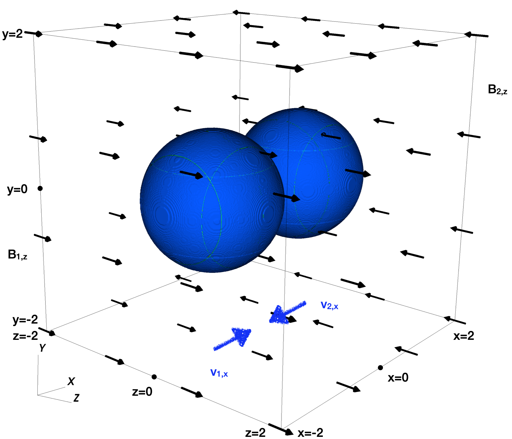
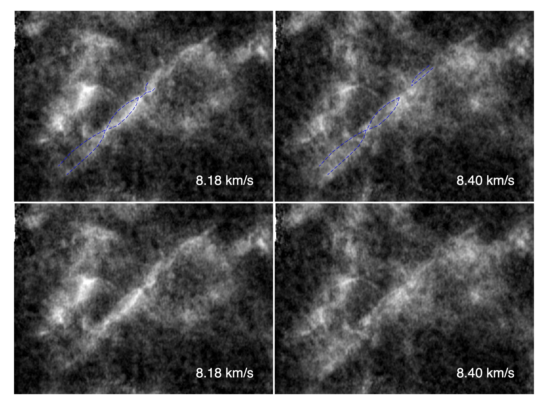
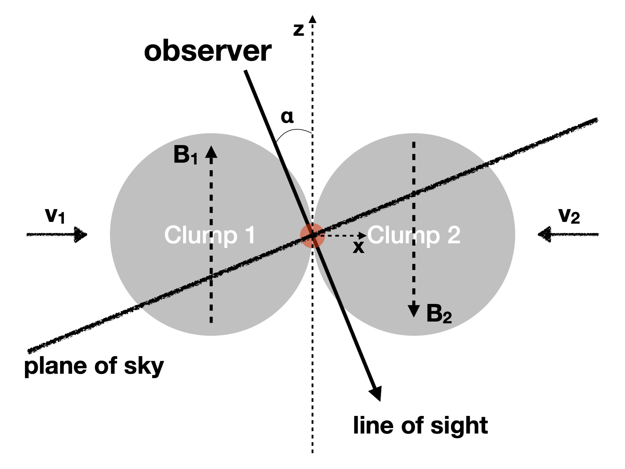
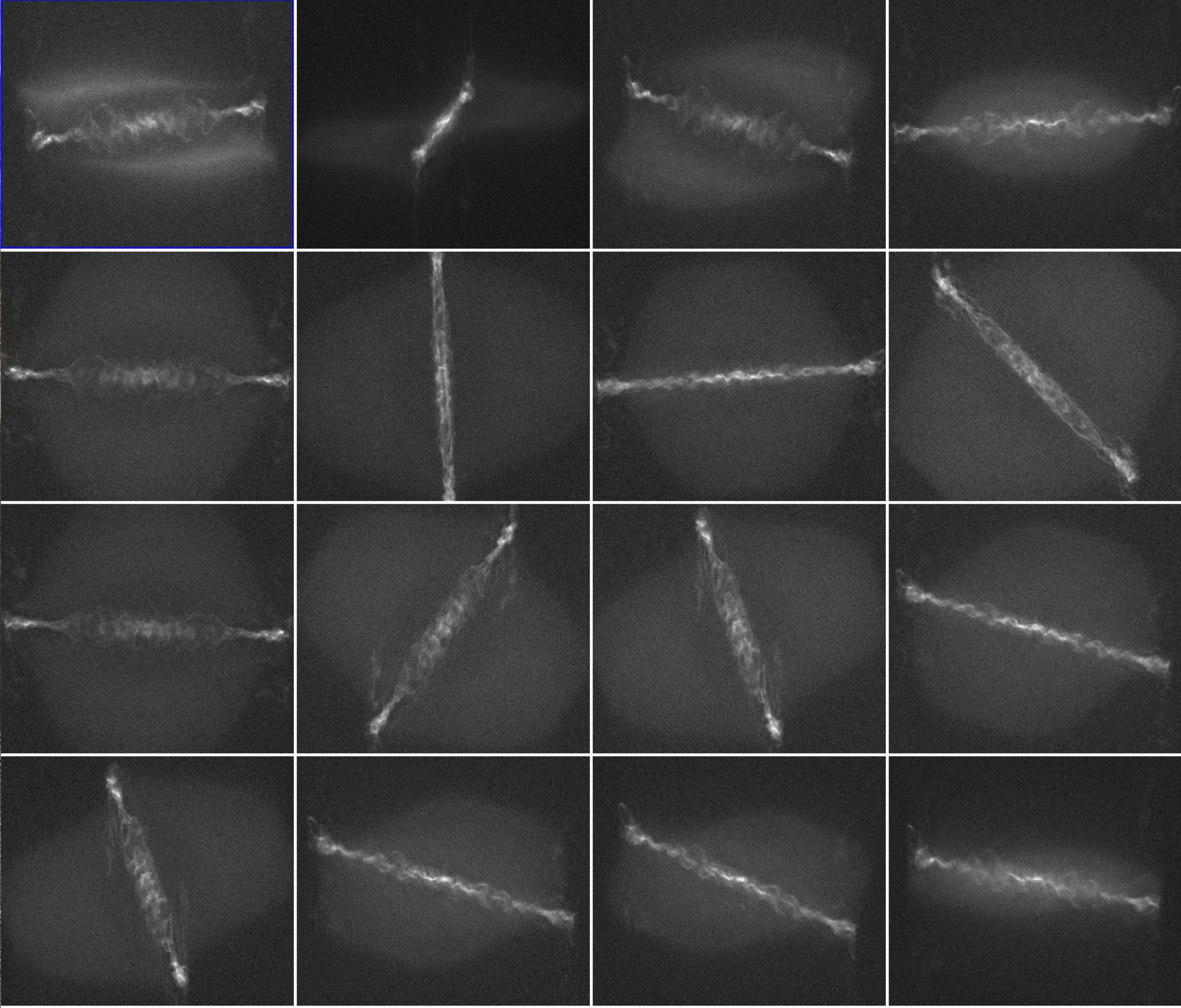
While going through the CARMA-NRO survey C¹⁸O data cube, I noticed a special filament (the Stick) at the southern end of the integral-shaped filament. It shows ring-like fibers at different velocity channels (see left column in the figure below). These ring-like fibers resemble those structures in magnetic reconnection simulations, which motivated me to model the filament formation in the context of magnetic reconnection. To my surprise, the 15-year-long effort by Dr. Carl Heiles who observed the HI Zeeman effect (Heiles (1997), ApJS, 111, 245) showed a reverse magnetic field on two sides of the Orion A cloud. This field-reversal is a necessary condition for CMR. Considering other observational facts such as the double-velocity spectral feature and the perpendicular plane-of-the-sky magnetic fields (e.g., Soler (2019), A&A, 629, 96), the only initial condition for the model is a setup like the right panel in the figure below. So I used the Athena++ code to set up a collision simulation between two spherical diffuse clouds (we always start with spheres:) with reverse magnetic fields (see the left panel in the top figure).

Surprisingly, instead of forming a compressed “pancake” structure, the collision resulted in the formation of a filament. This outcome contrasts with the intuitive expectation that a head-on collision between two spherical bodies would simply create a flattened structure at the center. However, a closer examination of a simulation slice revealed that a pancake did initially form. Soon after, it became wrapped by magnetic field loops, which exerted strong tension and gradually squeezed the pancake material toward the central axis, forming the filament. In other words, the filament formation does not need gravity! Although, gravity will take over with the growth of the filament mass, as long as the cloud collision continues.

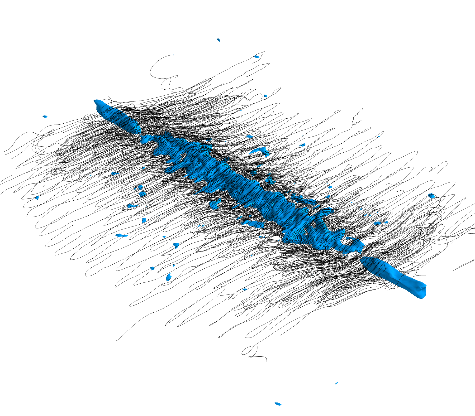
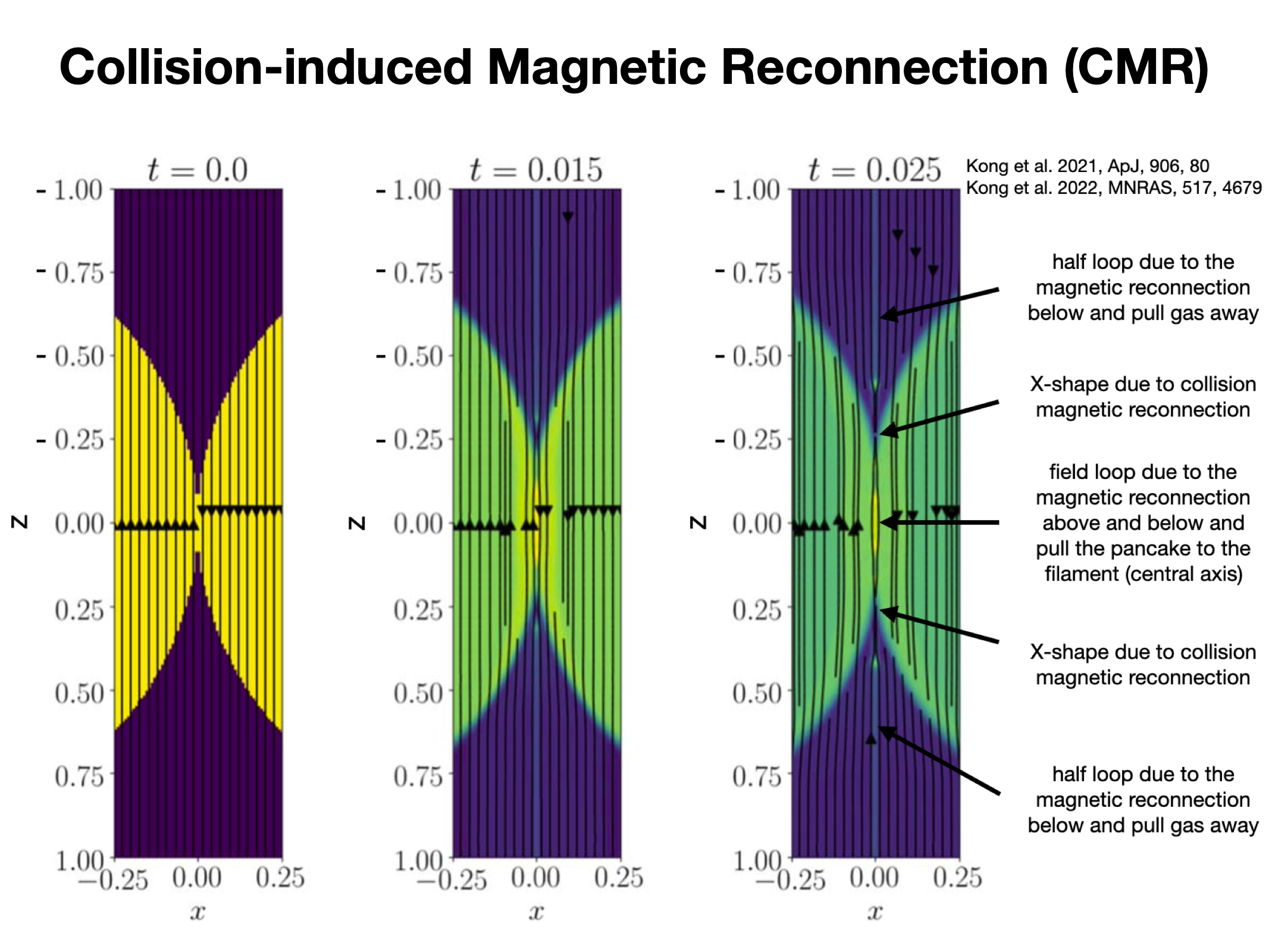
The figure below illustrates the formation of these magnetic loops. The collision triggered magnetic reconnection on both sides of the pancake, generating two half-loops and a full loop. The half-loops pulled gas outward, while the full loop compressed the pancake inward. As the collision progressed, ongoing reconnection continuously funneled dense gas into the central filament. This dynamic process is shown in the movie in the top figure.

Using the model filament, I performed synthetic observations and compared the resulting radiative transfer images with actual observational data. The model showed strong agreement with observed features, including the column density distribution, the position-velocity diagram, and overall morphological characteristics. Notably, it provided a natural explanation for the observed reversed magnetic field. An intriguing implication emerged from this analysis: the structures within the CMR filament appear to be confined by surface magnetic pressure. This finding aligns with the conclusion of Kirk et al. (2017), which suggests that dense cores in Orion are primarily pressure-confined.

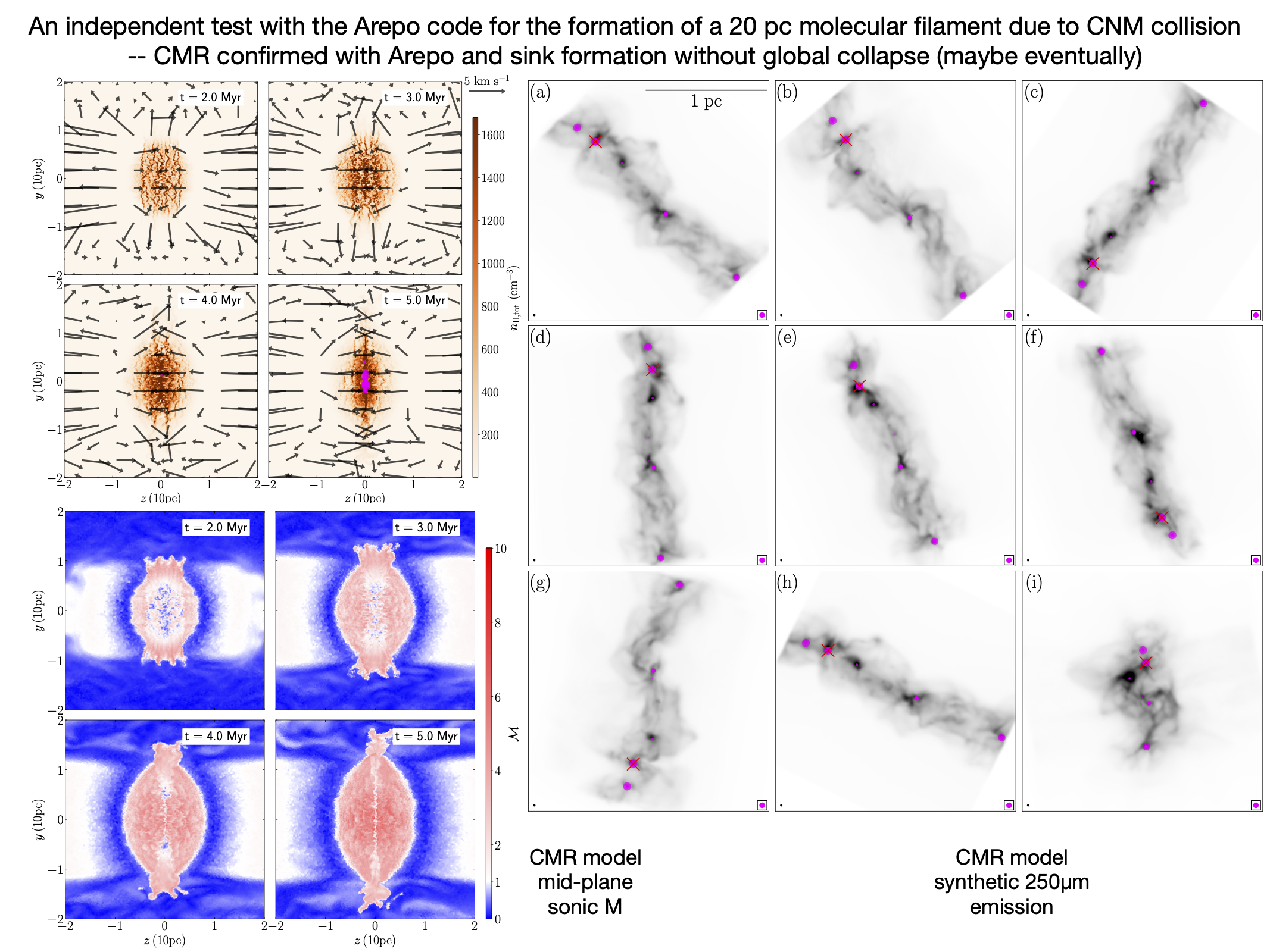
To investigate whether a filament like the Stick can form stars, we used the Arepo code with sink formation to repeat the above Athena++ simulation. First, the filament formation was reproduced in the Arepo simulation, so that CMR was independently confirmed with a different code. Second, the filament collapsed and formed a star cluster, but only after the filament became massive enough. An intriguing finding was that the star formation rate in CMR was a factor of two lower than a control model without CMR. The lower rate was due to the surface magnetic field that acted like a shield and hindered gas inflow. The result was reported in Kong et al. (2022), MNRAS, 517, 4679.

In Kong et al. (2023), ApJ, 265, 58, I led a brief parameter exploration of CMR to see how different initial conditions affect the filament property. Again, I used Athena++ for the simulations, following the 2021 Stick paper. A notable finding was that a curved filament would form if the initial colliding clouds have different radii or different density.

Using the exploration data, Dr. Duo Xu utilized machine-learning techniques to capture the morphological features of CMR filaments. Then, we applied the machine-learning models to the Herschel far infrared images of several filamentary clouds, including the Taurus cloud, the Orion cloud, and the Auriga–California Cloud. Several filamentary structures of these clouds were identified as CMR filaments. The findings were reported in Xu et al. (2023). Notably, these clouds were reported to have reverse magnetic fields (Tahani (2022)).

The MRCOL simulation began with molecular gas collision. A natural follow-up question is whether collisions between atomic gas can also lead to molecular cloud formation. In Kong et al. (2024), ApJ, 975, 97, we used Arepo again to model CMR within the cold neutral medium (CNM). The results showed that a filamentary molecular cloud successfully formed. This cloud exhibited numerous fiber-like substructures, with sinks actively accreting material through streamers. Recall from Kong et al. (2022), that sink accretion was only possible through streamers, as surface magnetic fields inhibited free gas inflow. Remarkably, this behavior persisted at a much larger scale (20 pc), with all sinks in the molecular cloud accreting via streamers. Most notably, the molecular cloud was naturally turbulent, driven by reconnected magnetic fields that funneled gas into the filament at supersonic (Alfvénic) speeds. This process compressed and transported shocked gas into the filament in a piece-by-piece manner. Consequently, filament formation in this scenario follows a bottom-up process -- distinct from the traditional top-down view of star formation, where gravity collects diffuse gas into a molecular cloud, which then collapses and fragments into clumps and cores. Remember, CMR filament formation proceeds without the need for gravity. In Kong (2022), ApJ, 933, 40, I also explored CMR in warm neutral medium in a disk galaxy.

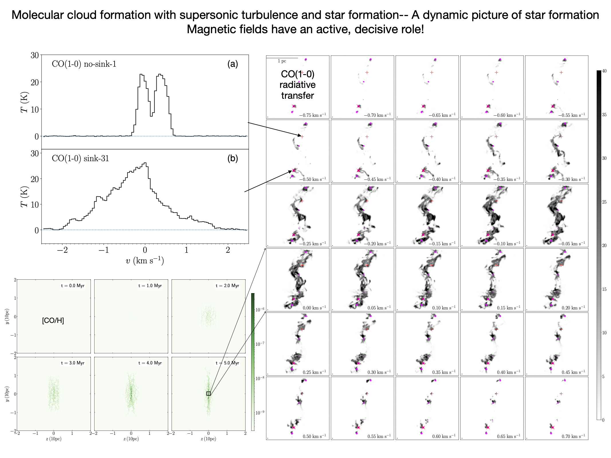
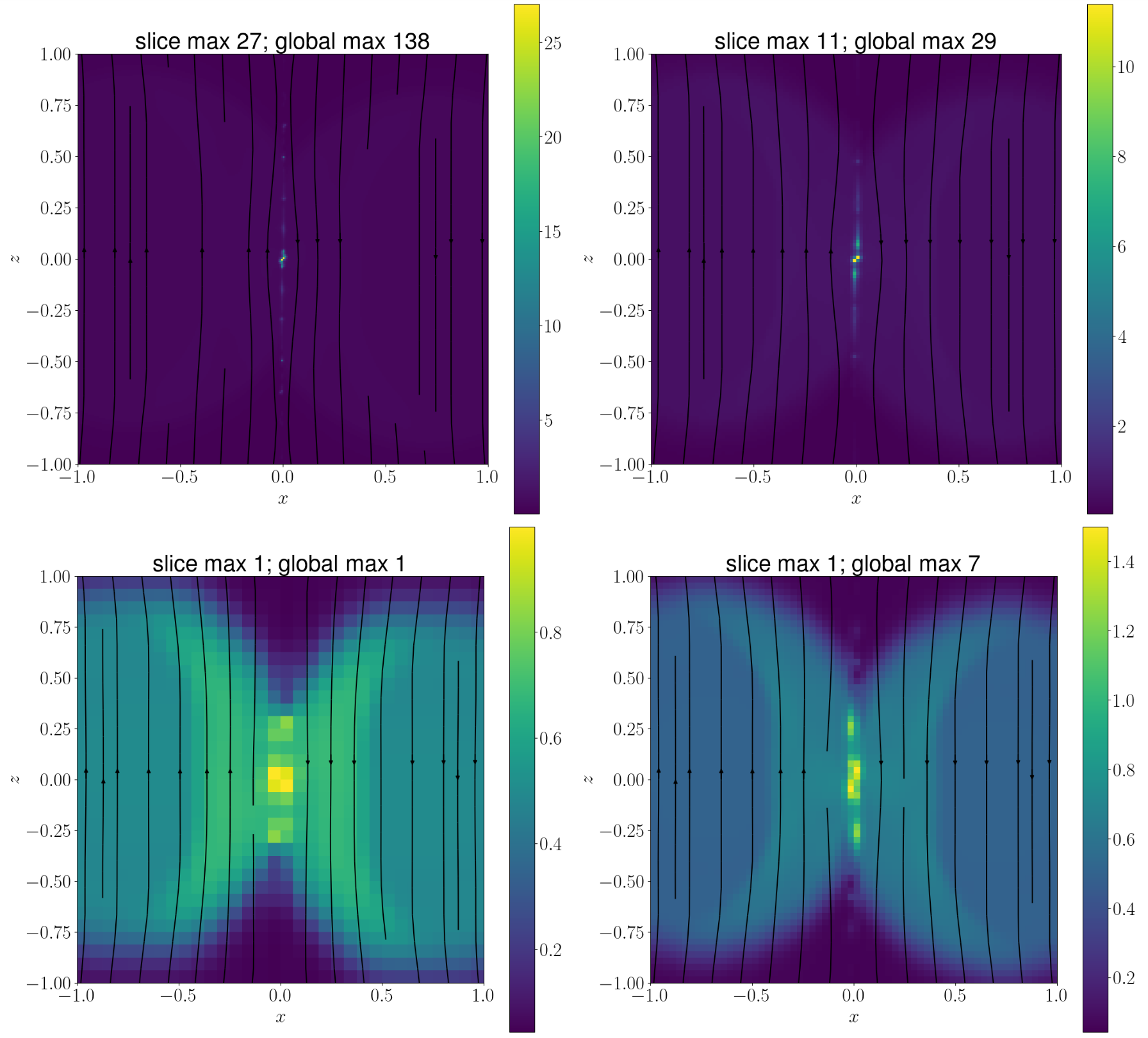
Recently, I revisit the MRCOL simulation to look for more testable observational features. In particular, I look into kinematic features to leverage the position-position velocity information provided by modern (sub-)mm molecular line observations. Using CO synthetic cubes, I find that CMR predicts two main kinematic features visible in position-velocity (PV) diagrams. The first is a transverse blueshift-redshift-blueshift-redshift (BRBR) pattern caused by a combination of converging gas motion toward the filament and diverging motion away from it. The pattern is a direct result of the combination of half-loop, full-loop, half-loop field pattern in the collision midplane (see the x-z slice plot above). The outflowing gas due to the half-loop is a typical feature of magnetic reconnection. The figure below illustrates the origin of the BRBR pattern.

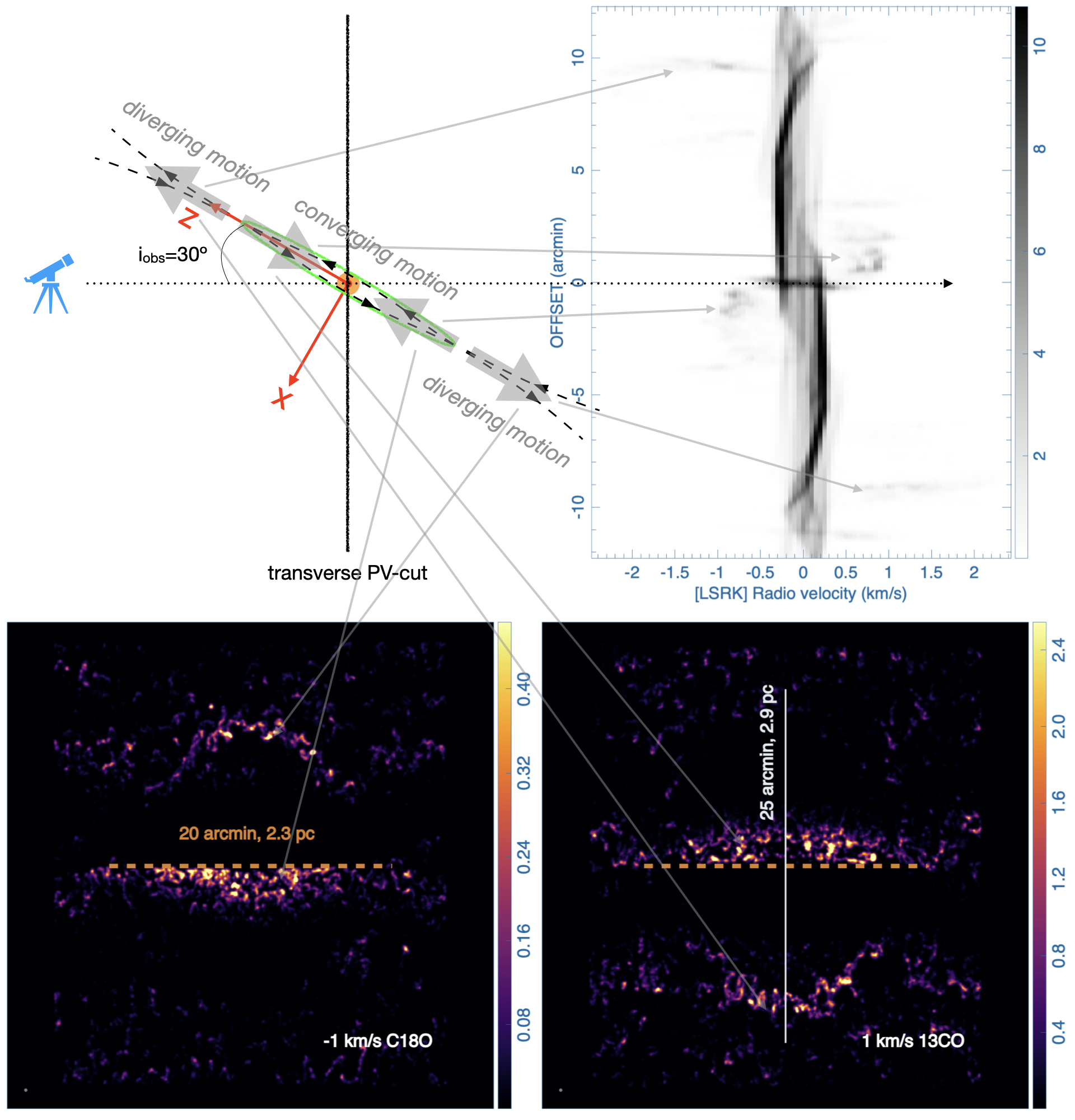
However, the BRBR feature primarily depends on emission outside the filament, which is difficult to confirm observationally because the signal is weak and easily confused with surrounding gas. I don't find a clear BRBR pattern around the Stick filament in the CARMA-NRO Orion data. So the usefulness of the BRBR pattern remains to be seen.

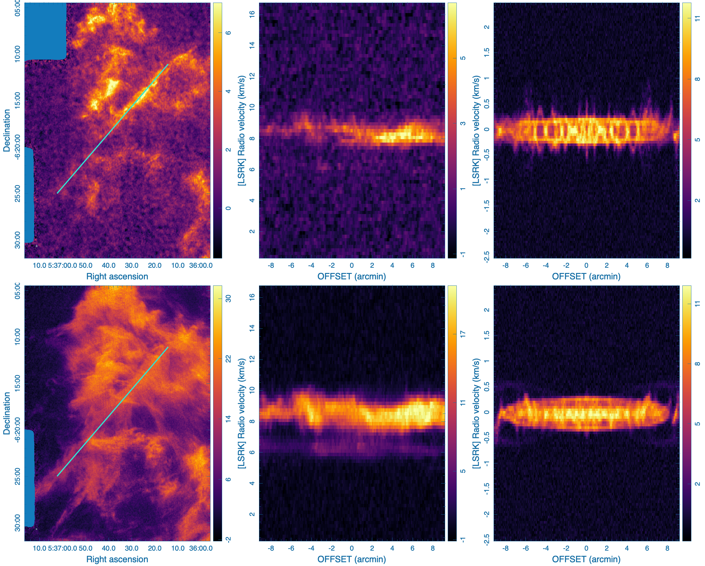
It turns out a velocity oscillation along the filament spine can be a better observational test for CMR. It appears as a zigzag pattern in longitudinal PV diagrams. This oscillation arises from clumpy gas being intermittently transported into the filament by magnetic tension, continuously stirring the filament. The figure below shows the pattern in both synthetic images and observation data.

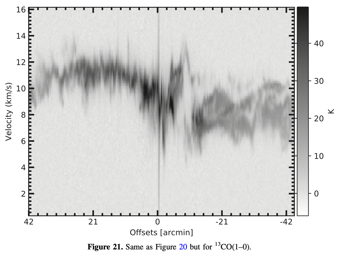
Interestingly, in the original CARMA-NRO Orion Survey paper Kong et al. (2018), ApJS, 236, 25, we found similar velocity oscillation along the spine of the integral-shaped filament in Orion A. The figure below shows an example of their ¹³CO PV-diagram (adapted from the paper). But see their other figures for ¹²CO and C¹⁸O. This is consistent with our suspect that Orion A formed via CMR. Interestingly, Poidevin et al. (2011) found evidence of a helical field around the OMC-1 filament, which is consistent with CMR.

Another interesting finding is that CMR filament has a typical diameter of ~0.02-0.1 pc in the fiducial setup of the model. The reason is that the filament cross-section is essentially the so-called plasmoid when folks in plasma physics study the plasmoid instability in magnetic reconnection. Based on studies in, e.g., Comisso et al. (2017), the size of a plasmoid can grow to typically a fraction of the current sheet length or a few times the current sheet thickness.

In the fiducial CMR simulation, the expected current sheet thickness (the thickness of the pancake) is ~ 0.02 pc. In the case of Sweet-Parker reconnection, the thickness δ_SP is approximately:

δ_SP ≈ L S_L^-1/2,

where L is the current sheet length and S_L is the Lundquist number:

S_L = L v_A / η

where v_A = B / √(4πρ) is the Alfvén speed and η is the Ohmic resistivity. In MRCOL, L is approximated by the length of the pancake, which is about the radius of the colliding clump. Therefore, in code unit, L = 0.9, v_A = 1.3, η = 0.001, thus S_L = 1170 and δ_SP = 0.026 which corresponds to 0.026 pc. If we set L as half the clump radius, then S_L = 585 and δ_SP = 0.019 pc. Therefore, the CMR-filament diameter should be somewhere between 0.02 pc to 0.1 pc. This implies that the diameter of CMR-filaments is largely determined by the property of the current sheet.

Interestingly, in my simulations, I remember that the ability to form the filament with a noticeable density increase depends on the simulation resolution, which was quite confusing to me at the time. Now it becomes clear: the simulation needs to resolve the current sheet thickness in order to see the formation of the filament. Otherwise, CMR happens but the filament is not prominent. The figure below shows a resolution-dependent change of the filament formation.